User's
quick guide to data location and extraction
Registering
as a user
To merely browse the inventory to inspect the
scope and extent of the data holdings, there is no need to register
nor to log-on for each browsing session.
To extract data, the user has to register (a
once-off activity). Without registration, data extraction will not
be possible. To register, click on 'registration' in the Home
Page.
After submission of the registration, the user is
informed of its acceptance by e-mail. Remember: direct extraction of
data is for research purposes only.
To browse the inventory (listings of data) or to
extract data, click on data
access button on the left. The user is first provided with a
brief description of what can be found on the Inventory.
By again clicking on 'Inventory and extraction' the user
is taken to the Inventory and extraction itself.
Return
to top
Locating data sets
The Inventory provides access to more than 6 000
individual data sets (a 'data set' being a cruise, or a deployed
instrument, etc).
In addition, there are more than 7 million records of
surface weather observations collected by Voluntary Observing Ships
(and therefore referred to as 'VOS'), since 1660. These can also be
accessed on-line (although not in the same way as the cruises).
It is often necessary to locate the survey you
are interested in (like a library book).
A user searches for a particular data set according to
the metadata of the survey (ship's name, date of the survey,
type of data, etc). These parameters are captured in the buttons
that appear on the left side of the screen in the Inventory (Fig.
1). A description of the functionality of these buttons is given
below.
Not all surveys have been supplied with a full array of
metadata, such as project name, chief scientist name, etc. The table
below
includes the % of entries that contain a particular metadata parameter.
The best parameters are date, vessel, or area, of which
the vessel
is most useful.
The location of a survey and its extraction are
illustrated
through a few examples. In many cases, use is made of drop-down
menus
since the database entries are sensitive to spelling.
 |
The SurveyID is not generally known
to the user up front and is therefore not really useful to search for a
cruise. The surveyID is a unique identifier of a data set, and includes
the year of loading (e.g. 2005) and a sequential number (e.g. 0007),
giving 2005/0007. Before 1990 the “year of loading” was
made the same as the year of the cruise. [100%]
|
 |
The date of the survey is always
available in the Inventory, but if a date is only roughly known by
the searcher (e.g. 1983), this search method can be used to start
from a certain date onwards (e.g. 1 Jan 1983) and identify the
required cruise from the other information supplied on screen.
[100%]
|
 |
A drop-down menu is provided to select the institute
name. Remember that some Institutes have, on occasion, changed names
over the years, so searching on this parameter is not unambiguous. [83%]
|
 |
This is useful if the scientist name
was provided at the time of data loading (not always the case, and not
for some historic data sets). [27%]
|
 |
The vessel name is normally a good
way to track down a data set. A number of cruises have been submitted
without a vessel name but these are largely ships-of-opportunity. [70%]
|
 |
By defining a lat/long area all the
surveys that had at least one station inside the box will be listed.
The full survey will then be identifiable. [100%]
|
 |
This option is useful for non-hydrographic (ship)
data (such as time series data
|
 |
Project names are loaded, where
available. Multiple names have also been loaded in the
“Project” field, and can be searched on any part of the
field (not just the start). [82%]
|
Fig. 1 Descriptions of the various
buttons by which the Inventory can be searched.
Note
- The total number of surveys in SADCO’s
inventory is 6 705 (June 2009).
- the percentage included in the table indicates the
portion of the total number of surveys that include that parameter
- shaded parameters are considered the best for
searching [date, vessel name, area], of which the vessel is most useful
Return
to top
Search
for data from an institute
By entering the first few characters of the Institute
name, an alphabetical list is provided of the institutes that start
with those characters.
In the example below (Fig. 2), 'nat' was entered, with
the intention to locate
'Natmirc' (National Marine Information and
Research Centre, Namibia)
By
selecting this institute from the drop-down list (Fig. 2), the next
page provides a list of years for which data from this institute is
available. If the number of surveys could fit on one screen, they
would be listed directly. If there are more (as in the present case
with 157 surveys), a further selection of the year is required (Fig. 3).
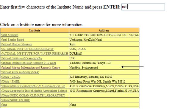
Fig. 2 The output after entering
“nat” for the Institute name.
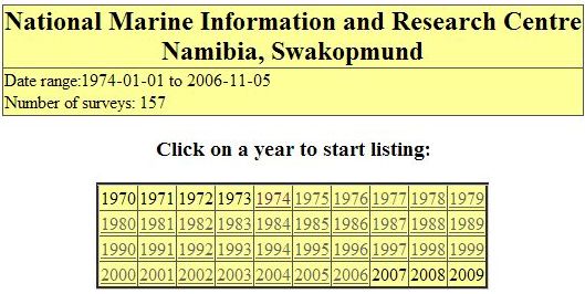
Fig. 3 After
selecting 'Natmirc' in Fig. 1, the year coverage of the 157
surveys executed by
Natmirc is provided (years marked in shading). Selection of a
particular year provides a listing of
the cruises
Fig. 4)
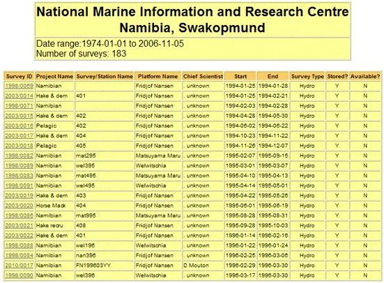
Fig. 4 Listing of NATMIRC cruises
obtained by clicking on '1994' in Fig. 3
Return
to top
Search
for data by scientist name
As before, enter the first few characters of the
scientist’s surname (without initials). In the example below, 'gor' was
entered and A L Gordon was selected from the list. The output is shown
in Fig. 5.
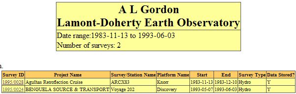
Fig. 5 List of the two cruises in which A L
Gordon was entered as the PI
Return
to top
Search
for data from a vessel (platform)
|
Enter the first few characters of the vessel
name. In the example on the right, 'mei' (first letters of 'Meiring
Naudé', the CSIR's research vessel, was entered.
The drop-down list (Fig. 6) shows Meiring Naudé at
the top, plus more vessels listed alphabetically. Click on 'Meiring
Naude', and this provides the output in Fig. 7.
From the Table in Fig. 7, '1975' was selected.
After selecting the year 1975, the output in Fig. 8 appears
Fig. 6 List of vessels
obtained after
entering 'mei' in the search field.
|
.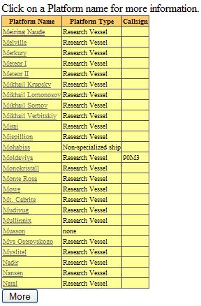 .. .. |
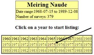
Fig. 7 Years during which the RV
Meiring Naudé executed 379 surveys
From the list in Fig. 8, the cruise with
the Survey_ID 1975/0043 (Project 'Bathy', Sept. 1975) was the one
selected. The final output of the Inventory is shown in Fig. 9a.
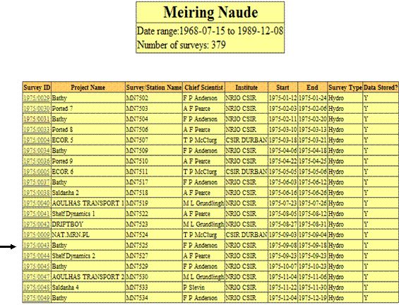
Fig. 8 List of Meiring Naudé cruises,
starting in 1975. The arrow indicates the 'Bathy'
cruise selected, and
portrayed in Fig. 9a
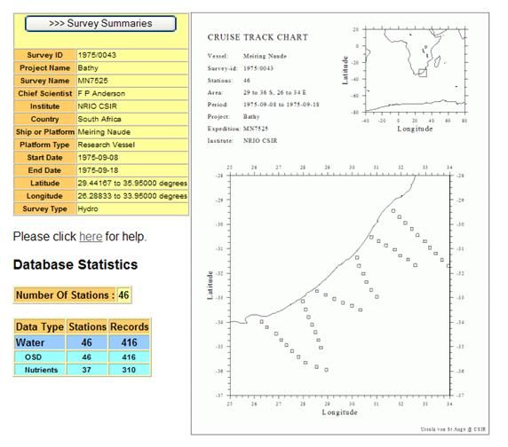
Fig. 9a. Metadata and track chart of the cruise of the 46 Meiring Naudé
stations on the
'Bathy' project in September 1975. 'OSD' refers to
discrete-level measurements (such as
bottles). Nutrients were sampled
on 37 stations, encompassing 310 individual samples.
If the user is registered and logged on,
the contents of Fig. 9a appear as shown below (Fig. 9b). By
clicking on the 'Extract on-line' button, the data is extracted and the
user informed by e-mail where to download the data.

Fig. 9b. Note that an 'extract online' button
appears at the bottom left when the user is
logged in. When clicked,
the data is extracted on-line without further ado, and the user
informed by e-mail where (= URL) the data can be viewed or downloaded.
Return
to top
Search
for time series data
Example A: Wave data. By clicking on the 'data
types' button, a drop-down menu appears from which the desired data
type can be selected (Fig. 10).
If 'hydro' is selected, the process becomes the same as shown above
(ship cruises).
Select 'Waves' and a list appears of wave stations of which data is
available (Fig. 11).
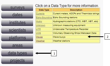
Fig. 10 Selecting the 'data types' search button (1) and the 'waves'
option (2) from
the drop-down menu.
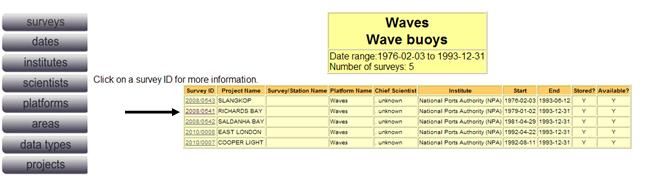
Fig. 11 Wave buoy stations for which data is in SADCO. Note that each
'survey'
covers a number of years.
Selection of Richards Bay from the
list,
shows the available data (Fig. 12), for the case where the user is
logged in. The column on the right indicates that the data can be
extracted on-line.
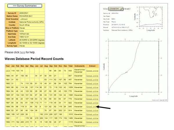
Fig. 12 Wave data available per year for the Richards
Bay wave buoy. Also indicated in
the year-month table is the instrument type. If the user
is logged in, a column is
visible
that indicates that the data can be extracted on-line (arrow)
Example B: weather data. Select 'Weather'
on the 'Data types' screen (Fig. 10), and click on Richards Bay
Port Control as an example. Fig. 13 shows the relevant outcome.
However, the amount of data for some years is now too high for direct
extraction. If such a set is selected by the user the request will be
routed to a SADCO staff member who will do the extraction and the user
is informed by e-mail.
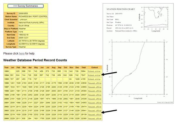
Fig. 13 Weather data available from
the Richards Bay Port Control weather station. The
top arrow indicates that the data can be extracted on-line (< 10 000
records) while the
bottom arrow indicates data that can only be extracted off-line (>
10 000 records).
Example C: current meter data. Click on
'Currents' in Fig. 10. The user is required to select a year, the same
as in Fig. 3 and 7. '1987' was selected in the present case. The
resulting list is shown in Fig. 14.
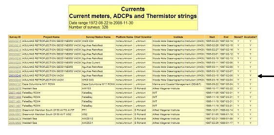
Fig. 14 List of current meter
deployments (moorings) that contained data during 1987.
The mooring indicated with an arrow was selected as an example, to
produce Fig. 15.
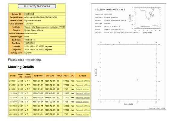
Fig. 15 Details of the mooring selected in Fig. 14. The
table shows that there were 3 instruments
on the mooring (at depths of 210m, 1 512m and 4 011m), the data of each
spanning 3 years (the
time series have been partitioned into years, and coloured). Some data
(marked 'Extract online')
can be extracted on-line, some will be handled off-line. All three
instruments recorded
temperature (T) and velocity (V), and one also recorded pressure (P).
Return
to top
Search
for data from a Project
If the project name was supplied to the data centre,
this could be a very useful search parameter. Because the correct
wording and spelling of project names are often not known to outside
users, the search according to Project Name compares the entered search
characters with the whole string in the 'Project' field, to find a hit
(not just the first few characters).
This allows for the possibility that the Project field in the data
centre may contain more than one Project name, such as
'ACEP/ASCLME/Agulhas Current System', and any of the projects will be
located during the search.
The output of a search for project 'Bathy' shows (Fig. 16) that 49 such
surveys were done. Picking a specific cruise from that table will
produce a similar output as in Fig. 9a or 9b.
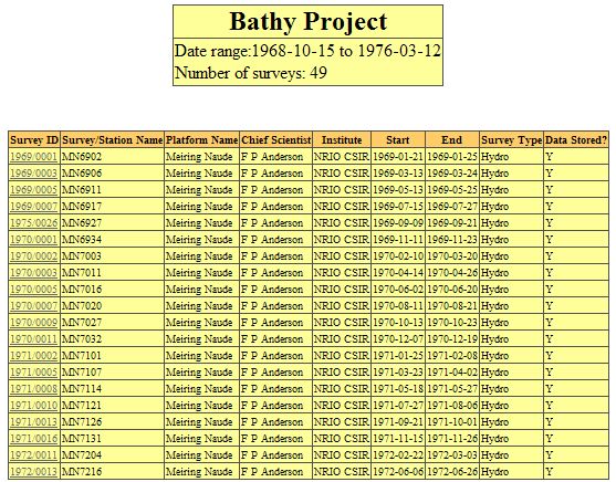
Fig. 16 List of cruises on the 'Bathy'
project, on which 49 surveys were
executed between 1968 and 1976.
Return
to top
Search for VOS
data
The Voluntary Observing Ships’ data comprises weather
observations made by ships of opportunity at so-called synoptic hours
(0:00, 6:00, 12:00, and 18:00). Parameters include sea surface
temperature, wind speed and direction; swell height and
direction, wind wave height, cloud cover, etc.
To access VOS data, select VOS from the menu in Fig. 10.
Because VOS data is not stored by survey, the selection is done by
lat-long rectangle and years (see Fig. 17). The on-line extraction must
be less than 100 rectangle degree-years. i.e. 10x10 degree for
1 year, 3x3 degrees for 10 years, etc. Fractions of a degree is allowed.
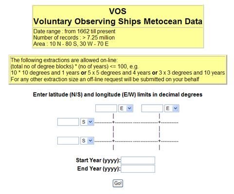
Fig. 17 Extraction method for VOS data. Because the data
is not collected or stored
by survey, the extraction is done by area
and period.
Return
to top
Queuing of requests
All requests are handled in tandem (= queued). If
it e.g. happens that a user’s request is #3 in the list, and requests
#1 and #2 take a couple of minutes each, request #3 will only start
being handled after a few minutes.
In case a given request 'hangs' (for some reason the extraction cannot
be executed), the request is removed from the queue after 10 minutes.
In such a case, the respective user is informed that the request will
be handled off-line and the other users in the queue are informed of
the delay.
Return
to top
Downloading
the extracted data
The e-mail sent to the user when the extraction is
complete includes the URL where the data can be downloaded. By (left)
clicking on the URL, the data will be listed for viewing. By
right-clicking, the user can indicate where the data should be saved.
Return
to top
Plotting the data
It is strongly suggested that the user obtain a copy of
ODV (Ocean Data View) which is freely available from
This is a powerful graphing programme that can produce
figures ready for inclusion in reports. Here is a quick introduction
just to get you started with ODV:
As an example, the data in Fig. 8b was extracted.
Opening with ODV
- Once the extracted data has been saved on your PC,
'open' the file with ODV (right-click on the file, select 'Open file
with…' and select ODV from the dropdown list.
- ODV will automatically import and plot the station
positions in one of its windows, and you’re ready to rock and roll. We
will show you only one of the many plotting options.
Defining the section (Fig. 18)
- Right-click somewhere on open space between the graph
templates on the screen, and select 'Layout templates' and then '1
section window' (this draws one section only).
- Right-click on the chart with plotted stations, then
select 'Manage section' and 'Define section'.
- The station chart enlarges (Fig. 18), to allow the
section to be defined
- A straight section can be defined by clicking on the
start position and double-clicking on the end position (or press Enter).
- A curved track can be created by successively
clicking along the desired route. Pressing 'Enter' ends the section.
- The section is not just a single line but an
enveloping box. If required, this box can be 'widened' in the
left-bottom box called 'Mean width'. Only stations within the envelope
will be plotted.
Setting up the graph (Fig. 19)
- Right-click on the section graph (which has now been
plotted) and set X variable (= distance), Y variable (= depth) and Z
variable (= temperature)
- Also select 'Set ranges' and adjust the scales
already entered there. E.g. temperature should be between 0 and
30 deg.
- At this stage, the section shows the depths where
measurements were taken (small dots), coloured according to the
temperature scale on the right. However, this is still not easy to
interpret.
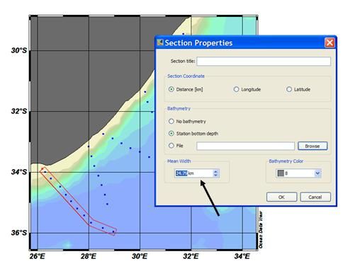
Fig. 18 Defining the section. The
width of the section can be widened by the
box indicated with the arrow
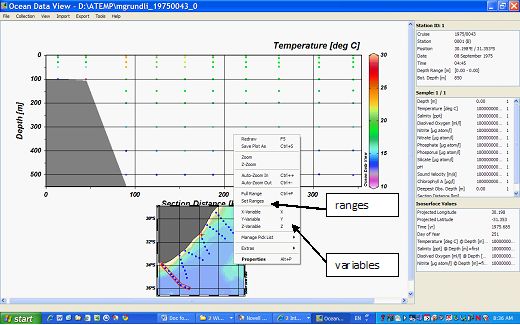
Fig. 19 On the same panel, the 'Draw marks' (this indicates the depths
where
measurements were taken) can be toggled (they are visible in Fig. 20c)
and the
size of the dots enlarged to be visible.
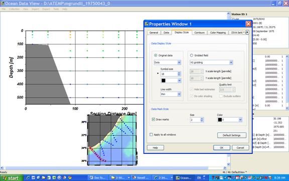
Fig. 20a Setting the contouring
options. This is the default screen for 'Display style'.The
measuring points are colour-coded according to the temperature scale.
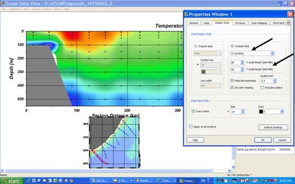
Fig. 20b Setting the contouring options. In the
'Display style' tab the 'Gridded field' has been
selected, and the gridding options set to 'VC gridding' and the X/Y
scale length modified.
The 'Draw marks' option is toggled, and the dot size enlarged.
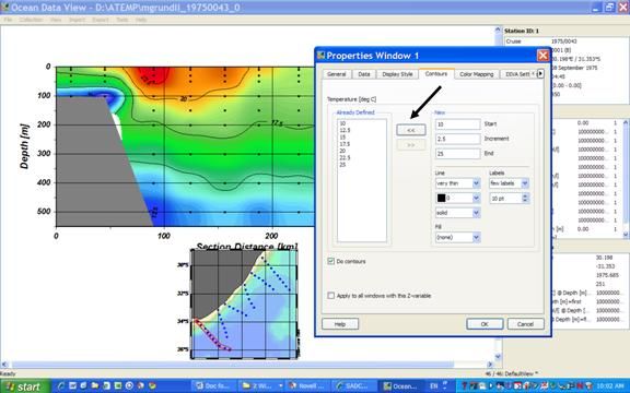
Fig. 20c Setting the contouring
options: In the 'Contours' tab, the contour intervals
(which were automatically created) have been transferred from right to
left with the
'<<' button. They are now visible on the graph.
Return
to top
|


")


